What are Saliency Maps?
Saliency maps is a technique to rank the pixels in an image based on their contribution to the final score from a Convolution Neural Network. The technique is described in great detail in this paper.
For e.g. if we have a ConvNet that gives a class score \(S_c(I)\) for an image \(I\) belonging to class \(c\). In a ConvNet the term \(S_c(I)\) is highly nonlinear but we can use the first-order Taylor expansion to approximate it as a linear function:
\[S_x(I) \approx w^TI + b\]where \(b\) is the bias and \(w\) defines the importance of the pixels in image \(I\) for the class \(c\)
\[w = \frac{\partial S_c}{\partial I}\]The derivative above provids us a class saliency map for image \(I\), the magnitude of \(w\) indicates which pixels need to be changed the least to affect the class score the most.
The original paper outlining this methodology is quite old at this point and their are already a couple of packages and blogs online that compute saliency maps but I have had trouble finding something that is compatible with Tensorflow 2.0.
So here I present how I computed saliency maps in Tensorflow 2.0.
Compute Saliency Maps Using Tensorflow 2.0
Load in the required packages and make sure that tensorflow version is >=2.0:
import tensorflow as tf
import tensorflow.keras as keras

import numpy as np
import matplotlib.pyplot as plt

print('tensorflow {}'.format(tf.__version__))
print("keras {}".format(keras.__version__))
tensorflow 2.1.0
keras 2.2.4-tf
In this example I will use the VGG16 model which you can load directly from Keras:
model = keras.applications.VGG16(weights='imagenet')
model.summary()
Model: "vgg16"
_________________________________________________________________
Layer (type)                 Output Shape              Param #
=================================================================
input_1 (InputLayer)         [(None, 224, 224, 3)]     0
_________________________________________________________________
block1_conv1 (Conv2D)        (None, 224, 224, 64)      1792
_________________________________________________________________
block1_conv2 (Conv2D)        (None, 224, 224, 64)      36928
_________________________________________________________________
block1_pool (MaxPooling2D)   (None, 112, 112, 64)      0
_________________________________________________________________
block2_conv1 (Conv2D)        (None, 112, 112, 128)     73856
_________________________________________________________________
block2_conv2 (Conv2D)        (None, 112, 112, 128)     147584
_________________________________________________________________
block2_pool (MaxPooling2D)   (None, 56, 56, 128)       0
_________________________________________________________________
block3_conv1 (Conv2D)        (None, 56, 56, 256)       295168
_________________________________________________________________
block3_conv2 (Conv2D)        (None, 56, 56, 256)       590080
_________________________________________________________________
block3_conv3 (Conv2D)        (None, 56, 56, 256)       590080
_________________________________________________________________
block3_pool (MaxPooling2D)   (None, 28, 28, 256)       0
_________________________________________________________________
block4_conv1 (Conv2D)        (None, 28, 28, 512)       1180160
_________________________________________________________________
block4_conv2 (Conv2D)        (None, 28, 28, 512)       2359808
_________________________________________________________________
block4_conv3 (Conv2D)        (None, 28, 28, 512)       2359808
_________________________________________________________________
block4_pool (MaxPooling2D)   (None, 14, 14, 512)       0
_________________________________________________________________
block5_conv1 (Conv2D)        (None, 14, 14, 512)       2359808
_________________________________________________________________
block5_conv2 (Conv2D)        (None, 14, 14, 512)       2359808
_________________________________________________________________
block5_conv3 (Conv2D)        (None, 14, 14, 512)       2359808
_________________________________________________________________
block5_pool (MaxPooling2D)   (None, 7, 7, 512)         0
_________________________________________________________________
flatten (Flatten)            (None, 25088)             0
_________________________________________________________________
fc1 (Dense)                  (None, 4096)              102764544
_________________________________________________________________
fc2 (Dense)                  (None, 4096)              16781312
_________________________________________________________________
predictions (Dense)          (None, 1000)              4097000
=================================================================
Total params: 138,357,544
Trainable params: 138,357,544
Non-trainable params: 0
_________________________________________________________________
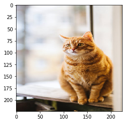
Load the image that you want to run the model on:
_img = keras.preprocessing.image.load_img('cat_front.jpeg',target_size=(224,224))
plt.imshow(_img)
plt.show()
The image we have loaded needs to be preprocessed before we can submit it to the model and get the class scores. The last layer of the VGG16 model gives a score for each class. Run the model to get the predictions.
#preprocess image to get it into the right format for the model
img = keras.preprocessing.image.img_to_array(_img)
img = img.reshape((1, *img.shape))
y_pred = model.predict(img)
The highest class score is at index 285, which is equivalent to an Egyptian Cat (see here). We can calculate the gradient with respect to the top class score to see which pixels in the image contribute the most:
images = tf.Variable(img, dtype=float)

with tf.GradientTape() as tape:
    pred = model(images, training=False)
    class_idxs_sorted = np.argsort(pred.numpy().flatten())[::-1]
    loss = pred[0][class_idxs_sorted[0]]

grads = tape.gradient(loss, images)
dgrad_abs = tf.math.abs(grads)
To get the saliency map we need to find the max of the absolute values of the gradient along each RGB channel
dgrad_max_ = np.max(dgrad_abs, axis=3)[0]
Normalize the grad to between 0 and 1
## normalize to range between 0 and 1
arr_min, arr_max  = np.min(dgrad_max_), np.max(dgrad_max_)
grad_eval = (dgrad_max_ - arr_min) / (arr_max - arr_min + 1e-18)
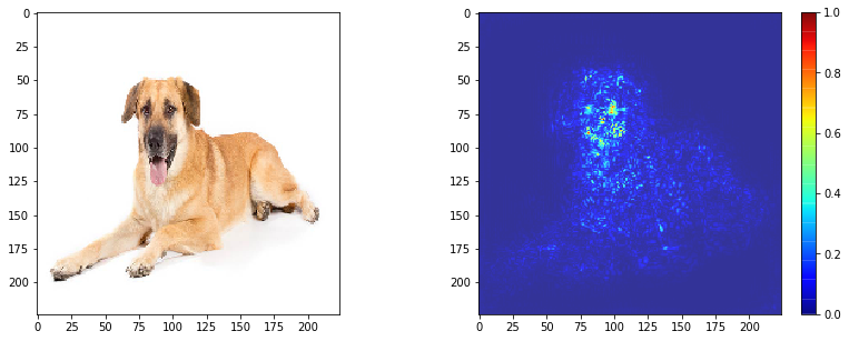
The output will look as follows:
fig, axes = plt.subplots(1,2,figsize=(14,5))
axes[0].imshow(_img)
i = axes[1].imshow(grad_eval,cmap="jet",alpha=0.8)
fig.colorbar(i)
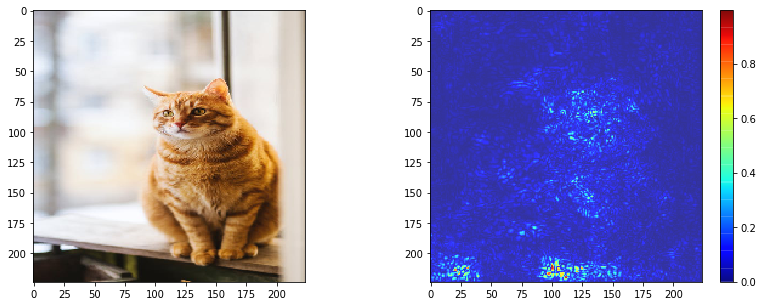
The cats face, background near the paws and some background on the bottom-left contribute the most to its top class score.
Check out the full notebook here
References
- Fairyonice.github.io. 2020. Saliency Map With Keras-Vis. [online] Available at: https://fairyonice.github.io/Saliency-Map-with-keras-vis.html [Accessed 2 May 2020].
- https://arxiv.org/abs/1312.6034v2
Comments