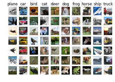
In this exercise we are asked to train a k-NN classifier on the CIFAR-10 dataset. The CIFAR-10 dataset consists of 60000 32x32 colour images in 10 classes, with 6000 images per class. There are 50000 training images and 10000 test images.
Using Two Loops to Calculate Distances
This is rather simple, we need to calculate the Euclidean distance between each point in our testing and training dataset. We have already reshaped the CIFAR-10 data into single rows. So the distance between test data i and train data j is given as
\[\begin{align} dist[i,j] = \sqrt{(\sum_{dim=1}^{dim=3072} (X\_train[j][dim] - X\_ test[i][dim])^2} \end{align}\]Another way to write this as a dot product:
\[\begin{align} dist[i,j] = \sqrt{(X\_ train[j] - X\_test[i]) \cdot (X\_ train[j] - X\_test[i])} \end{align}\]Here is the code implemented in python:
num_test = X.shape[0]
num_train = self.X_train.shape[0]
dists = np.zeros((num_test, num_train))
for i in range(num_test):
    for j in range(num_train):
        v_sub = X[i] - self.X_train[j]
        dists[i, j] = np.sqrt(v_sub.dot(v_sub))
This is what the distance matrix between the training (X-axis) and testing set (Y-axis) looks like.

The bright in the image above indicate test images that are very similar to a variety of training images based on a simple Euclidean distance. This would also imply that the image classification for the images with bright rows will not be very reliable.
Similarly for bright columns, the training images would be very similar to all images in the test set based on simple Euclidean distance.
Using One Loop to Calculate Distances
We can use some numpy magic to calculate the distance matrix with just one loop
num_test = X.shape[0]
num_train = self.X_train.shape[0]
dists = np.zeros((num_test, num_train))
for i in range(num_test):
    v_sub = self.X_train - X[i]
    dists[i] = np.sqrt(np.sum(v_sub**2, axis=1))
Using No Loop to Calculate Distances
We can simplify the calculation even further to the point where we don’t need to use any loops.
\[\begin{align*} dist &= \begin{pmatrix} (X\_train[0] - X\_test[0]) \cdot (X\_train[0] - X\_test[0]) & (X\_train[1] - X\_test[0]) \cdot (X\_train[1] - X\_test[0]) & \dots & (X\_train[5000] - X\_test[0]) \cdot (X\_train[5000] - X\_test[0]) \\ (X\_train[0] - X\_test[1]) \cdot (X\_train[0] - X\_test[1]) & (X\_train[1] - X\_test[1]) \cdot (X\_train[1] - X\_test[1]) & \dots & (X\_train[5000] - X\_test[1]) \cdot (X\_train[5000] - X\_test[1]) \\ \vdots & \vdots & \ddots \\ (X\_train[0] - X\_test[500]) \cdot (X\_train[0] - X\_test[500]) & (X\_train[1] - X\_test[500]) \cdot (X\_train[1] - X\_test[500]) & \dots & (X\_train[5000] - X\_test[500]) \cdot (X\_train[5000] - X\_test[500])\\ \end{pmatrix} \end{align*}\]Rewrite the matrix multiplication above as follows
\[\begin{align*} dist = \begin{pmatrix} X\_train[0] \cdot X\_train[0] & X\_train[1] \cdot X\_train[1] & \dots & X\_train[5000] \cdot X\_train[5000] \\ X\_train[0] \cdot X\_train[0] & X\_train[1] \cdot X\_train[1] & \dots & X\_train[5000] \cdot X\_train[5000] \\ \vdots & \vdots & \ddots \\ X\_train[0] \cdot X\_train[0] & X\_train[1] \cdot X\_train[1] & \dots & X\_train[5000] \cdot X\_train[5000]\\ \end{pmatrix} \\ + \begin{pmatrix} X\_test[0] \cdot X\_test[0] & X\_test[0] \cdot X\_test[0] & \dots & X\_test[0] \cdot X\_test[0] \\ X\_test[1] \cdot X\_test[1] & X\_test[1] \cdot X\_test[1] & \dots & X\_test[1] \cdot X\_test[1] \\ \vdots & \vdots & \ddots \\ X\_test[500] \cdot X\_test[500] & X\_test[500] \cdot X\_test[500] & \dots & X\_test[500] \cdot X\_test[500]\\ \end{pmatrix}\\ -2*\begin{pmatrix} X\_train[0] \cdot X\_test[0] & X\_train[1] \cdot X\_test[0] & \dots & X\_train[5000] \cdot X\_test[0] \\ X\_train[0] \cdot X\_test[1] & X\_train[1] \cdot X\_test[1] & \dots & X\_train[5000] \cdot X\_test[1] \\ \vdots & \vdots & \ddots \\ X\_train[0] \cdot X\_test[500] & X\_train[1] \cdot X\_test[500]) & \dots & X\_train[5000] \cdot X\_test[500]\\ \end{pmatrix} \end{align*}\]This is not the most intuitive way to think about this but we can actually use numpy to do the matrix calculations above in a single line.
dists = (self.X_train**2).sum(axis=1) + (X**2).sum(axis=1)[:, np.newaxis] - 2*X.dot(self.X_train.T)
Here is how long each version of the code takes to run on the CIFAR-10 dataset:
Two loop version took 21.103897 seconds
One loop version took 39.334489 seconds
No loop version took 0.198159 seconds
As stated in the assignment notes:
# NOTE: depending on what machine you're using,
# you might not see a speedup when you go from two loops to one loop,
# and might even see a slow-down.
Check out the full assignment here
Comments