Fully-Connected Layers – Forward and Backward
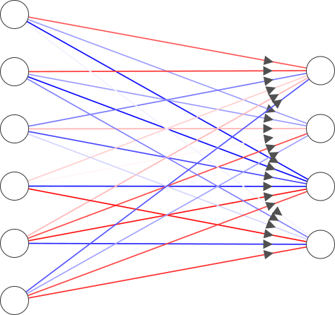
A fully-connected layer is in which neurons between two adjacent layers are fully pairwise connected, but neurons within a layer share no connection.
 Fully-connected layers (biases are ignored for clarity). Made using NN-SVG
Forward
In a fully-connected neural network inputs from the incoming layer is transformed to next layer via matrix multiplication. For e.g., the incoming neurons of layer \(\mathbf{x}\) are transformed to the neurons of the next layer \(\mathbf{out}\) as
\[\begin{align} \mathbf{out} = \mathbf{x} \cdot \mathbf{W} + \mathbf{b} \end{align}\]where
\[\begin{align} \mathbf{out} = \begin{pmatrix} h^{(2)}_{1} & h^{(2)}_{2} & \dots & h^{(2)}_{k} \end{pmatrix} , \\ \nonumber \\ \mathbf{x} = \begin{pmatrix} h^{(1)}_{1} & h^{(1)}_{2} & \dots & h^{(1)}_{l} \end{pmatrix}, \nonumber \\ \mathbf{W} = \begin{pmatrix} W_{1,1} & W_{1,2} & \dots & W_{1,k} \\ W_{2,1} & W_{2,1} & \dots & W_{2,k} \\ \vdots & \vdots & \ddots & \vdots \\ W_{l,1} & W_{l,2} & \dots & W_{l,k} \\ \end{pmatrix}, \nonumber \\ \mathbf{b} = \begin{pmatrix} b_{1} & b_{2} & \dots & b_{k} \end{pmatrix} \end{align}\]In Python,
def affine_forward(x, w, b):
    num_inputs = x.shape[0]
    input_shape = x.shape[1:]
    output_dim = b.shape[0]

    # reshaping to flatten the RGB image from CIFAR-10 dataset
    out = x.reshape(num_inputs, np.prod(input_shape)).dot(w) + b
    cache = (x, w, b)
    return out, cache
Backward
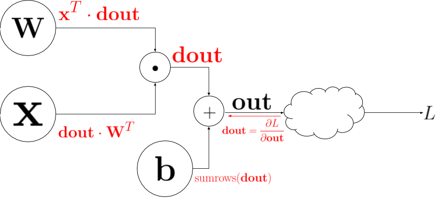
For the backward pass over the fully connected layers we need to calculate the gradient of \(\mathbf{out}\) with respect to \(\mathbf{W}, \mathbf{x}\) and \(\mathbf{b}\). Lets take at a look at the circuit diagram representing the fully-connected neural layers.
 Circuit diagram for fully-connected layers. The backprop derivatives are shown in red.
In Python, we can write the backward pass as follows:
def affine_backward(dout, cache):
    x, w, b = cache

    num_inputs = x.shape[0]
    input_shape = x.shape[1:]
    output_dim = b.shape[0]

    dx = dout.dot(w.T)
    # reshaping to flatten the RGB image from CIFAR-10 dataset
    dx = dx.reshape(x.shape)
    dw = x.reshape(num_inputs, np.prod(input_shape)).T.dot(dout)
    db = np.sum(dout, axis = 0)

    return dx, dw, db
ReLU Activation
ReLU stands for rectified linear activation function. It is a commonly used activation function that is used throughout this notebood. Mathematically the forward and backward pass over ReLU activation is quite simple to understand and implement. Here is the ReLU activation function forward pass:
\[\begin{align}\label{eqn:ReLU} y = \begin{cases} x, \text{if } x > 0 \\ 0, \text{otherwise} \end{cases} \end{align}\]Using numpy we can implement it as follows in Python:
def relu_forward(x):
    out = np.maximum(x, 0)

    cache = x
    return out, cache
For the backward pass take the derivative of Eq. \ref{eqn:ReLU} with respect to x:
\[\begin{align} \frac{\partial y}{\partial x} = \begin{cases} 1, \text{if } x > 0 \\ 0, \text{otherwise} \end{cases} \end{align}\]This can also be easily implemented using numpy:
def relu_backward(dout, cache):
    dx, x = None, cache
    dx = np.where(x>=0, 1, 0)
    # need to multiply by the incoming upstream derivative
    dx = dout*dx

    return dx
Two-Layer Fully Connected Neural Network
I have already covered the Two-Layer Fully Connected Neural Network here, so I am not going to repeat myself. We can modify the code that we already have and use the modular approach to write cleaner code.
class TwoLayerNet(object):
    def __init__(self, input_dim=3*32*32, hidden_dim=100, num_classes=10,
                 weight_scale=1e-3, reg=0.0):

        self.params = {}
        self.reg = reg

        self.params['W1'] = np.random.normal(0, weight_scale, (input_dim, hidden_dim))
        self.params['b1'] = np.zeros(hidden_dim)

        self.params['W2'] = np.random.normal(0, weight_scale, (hidden_dim, num_classes))
        self.params['b2'] = np.zeros(num_classes)

        self.input_dim = input_dim
        self.hidden_dim = hidden_dim
        self.num_classes = num_classes

    def loss(self, X, y=None):

        scores = None

        N = X.shape[0]

        # first layer activation
        H_1, cache_H1 = affine_forward(X, self.params['W1'], self.params['b1'])
        A_1, cache_relu = relu_forward(H_1)


        # second layer activation
        scores, cache_scores = affine_forward(A_1, self.params['W2'], self.params['b2'])

        # If y is None then we are in test mode so just return scores
        if y is None:
            return scores

        loss, grads = 0, {}

        loss, grad_L_wrt_scores = softmax_loss(scores, y)
        loss += 0.5 * self.reg * (
                    np.sum(self.params['W1'] * self.params['W1']) + np.sum(self.params['W2'] * self.params['W2']))

        grad_L_wrt_A_2, grad_L_wrt_W2, grad_L_wrt_b2 = affine_backward(grad_L_wrt_scores, cache_scores)

        grad_L_wrt_H_1 = relu_backward(grad_L_wrt_A_2, cache_relu)

        grad_L_wrt_X, grad_L_wrt_W1, grad_L_wrt_b1 = affine_backward(grad_L_wrt_H_1, cache_H1)

        grads['W1'] = grad_L_wrt_W1 + self.reg * self.params['W1']
        grads['b1'] = grad_L_wrt_b1
        grads['W2'] = grad_L_wrt_W2 + self.reg * self.params['W2']
        grads['b2'] = grad_L_wrt_b2

        return loss, grads
Multilayer Network
Creating a multilayer neural network of arbitray length is easy with the modular approach. A multilayer fully-connected neural network is made up of smaller fully-connected neural network.
To start, initialize the weights for the neural network:
# first layer weights
self.params['W1'] = np.random.normal(0, weight_scale, [input_dim, hidden_dims[0]])
self.params['b1'] = np.zeros([hidden_dims[0]])

# hidden layer
for i in range(2, self.num_layers):
    self.params['W' + str(i)] = np.random.normal(0, weight_scale, [hidden_dims[i - 2], hidden_dims[i - 1]])
    self.params['b' + str(i)] = np.zeros([hidden_dims[i - 1]])

# the final layer
self.params['W' + str(self.num_layers)] = np.random.normal(0, weight_scale,
                                                           [hidden_dims[self.num_layers - 2],
                                                            num_classes])
self.params['b' + str(self.num_layers)] = np.zeros([num_classes])
Now the forward pass
# first layer
self.cache['H1'], self.cache['cache_H1'] = affine_forward(X, self.params['W1'], self.params['b1'])
#ReLU
self.cache['A1'], self.cache['cache_A1'] = relu_forward(self.cache['H1'])

#Intermediate hidden laters
for i in range(2, self.num_layers):
    self.cache['H' + str(i)], self.cache['cache_H' + str(i)] = affine_forward(
    self.cache['A' + str(i - 1)], self.params['W' + str(i)], self.params['b' + str(i)])

    self.cache['A' + str(i)], self.cache['cache_A' + str(i)] = relu_forward(self.cache['H' + str(i)])

# output layer
scores, self.cache['cache_H' + str(self.num_layers)] = affine_forward(self.cache['A' + str(self.num_layers - 1)],
                                      self.params['W' + str(self.num_layers)],
                                      self.params['b' + str(self.num_layers)] )
For the backward pass we can use the cache variable created in the affine_forward and ReLU_forward function to compute affine_backward and ReLU_backward. For e.g. a 2 layer neural network would look like this:
 Using the inputs to the forward passes in backward pass.
In python within the framework of the assignment it can be implemented in the following way:
# first backward pass
loss, grad_L_wrt_scores = softmax_loss(scores, y)
for i in range(1, self.num_layers + 1):
    loss += 0.5 * self.reg * (np.sum(self.params['W' + str(i)] * self.params['W' + str(i)]) )


backward = {}

backward['A' + str(self.num_layers - 1)], grads['W' + str(self.num_layers)], \
grads['b' + str(self.num_layers)] = affine_backward(grad_L_wrt_scores,
                                        self.cache['cache_H' + str(self.num_layers)])

grads['W' + str(self.num_layers)] += self.reg*self.params['W' + str(self.num_layers)]

for i in range(self.num_layers - 1, 0, -1):
    backward['H' + str(i)] = relu_backward(backward['A' + str(i)], self.cache['cache_A' + str(i)])

    backward['A' + str(i - 1)], grads['W' + str(i)], grads['b' + str(i)] = affine_backward(
                                    backward['H' + str(i)], self.cache['cache_H' + str(i)])

## A0 corresponds to dX

    grads['W' + str(i)] += self.reg*self.params['W' + str(i)]
Check out the full assignment here
Comments