Autoregressive Model -- Properties of AR(1) Model

Photo by Annie Spratt on Unsplash

An autoregressive (AR) model predicts the future value based on previous values. Before jumping into the math behind AR models, we need to discuss a concept called stationarity.

Stationarity

A time series is stationary if its properties are independent of the times at which the time series is observed. For e.g. the properties of the stationary time series ($r_{t_1}, …, r_{t_k}$) is identical to that of ($r_{t_1+1}, …, r_{t_k+1}$) for all $t$.

More specifically, a time series ($r_{1}, r_{2}, …, r_{t}$) is stationary if

$$E[r_t] = \mu$$

for all $t$,

$$\text{Cov}(r_{t}, r_{r-l})=\gamma_{l}$$

which only depends on $l$.

Autoregressive Models

Now lets get back to AR models. An AR($p$) is written as follows

$$y_{t} = \phi_{0} + \phi_{1}y_{t-1} + \phi_{2}y_{t-2} + ... + \phi_{p}y_{t-p} + \epsilon_{t}$$

where $\epsilon_{t}$ is white noise with E[$\epsilon_{t}$] = 0 and Var[$\epsilon_{t}$] = $\sigma^2$

AR(1) Model

Now lets look at AR(1) model in detail

$$\begin{align} \label{eqn:ar1} y_{t} = \phi_{0} + \phi_{1}y_{t-1} + \epsilon_{t} \end{align}$$

Taking the expectation of this equation

$$\begin{align} E[y_{t}] &= E[\phi_{0} + \phi_{1}y_{t-1} + \epsilon_{t}] \nonumber \\ \mu &= E[\phi_{0}] + E[\phi_{1}y_{t-1}] + E[\epsilon_{t}] \nonumber \\ &= E[\phi_{0}] + \phi_{1}E[y_{t-1}] + E[\epsilon_{t}] \nonumber \\ &= \phi_{0} + \phi_{1}\mu \end{align}$$

Solving for $\mu$ we get

$$\begin{align} \label{eqn:mu_ar1} \mu = \frac{\phi_{0}}{1-\phi_{1}} \end{align}$$

Now, lets take the variance of Eq. $\ref{eqn:ar1}$

$$\begin{align} \text{Var}[y_{t}] &= \text{Var}[\phi_{0} + \phi_{1}y_{t-1} + \epsilon_{t}] \nonumber \\ &= \text{Var}[\phi_{0}] + \text{Var}[\phi_{1}y_{t-1}] + \text{Var}[\epsilon_{t}] \nonumber \\ &= \phi_{1}^2\text{Var}[y_{t-1}] + \sigma^{2} \end{align}$$

using the property of stationarity ($\text{Var}[y_{t}] =\text{Var}[y_{t-1}]$)

$$\text{Var}[y_{t}] = \frac{\sigma^{2}}{1 - phi_{1}^2}$$

notice that $\phi_{1}^2$ < 1, because varaince needs to finite and is by definition nonnegative.

We can rearrange Eq. $\ref{eqn:mu_ar1}$ to get

$$\phi_{0} = (1 - \phi_{1})\mu$$

and rewrite Eq. $\ref{eqn:ar1}$ as

$$\begin{align} y_{t} &= \phi_{0} + \phi_{1}y_{t-1} + \epsilon_{t} \nonumber \\ &= (1 - \phi_{1})\mu + \phi_{1}y_{t-1} + \epsilon_{t} \end{align}$$

We can rewrite the equation above as

$$\begin{align} y_{t} - \mu &= -\phi_{1}\mu + \phi_{1}y_{t-1} + \epsilon_{t} \nonumber \\ &= \phi_{1}(y_{t-1} - \mu) + \epsilon_{t} \end{align}$$

Autocorrelation Fucntion of AR(1) Model

The correlation between two random variable $X$ and $Y$ is defined as

$$\begin{align} \rho_{x,y} &= \frac{\text{Cov}[X,Y]}{\sqrt{\text{Var}[X] \text{Var}[Y] }} \nonumber \\ &= \frac{ E[(X-\mu_{x}) (Y-\mu_{y}) )] }{\sqrt{ E[(X-\mu_{x})^2] E[(Y-\mu_{y})^2] }} \end{align}$$

Let

$$\begin{align} \rho_{l} &= \frac{\text{Cov}[y_{t},y_{t-l}]}{\sqrt{\text{Var}[y_{l}] \text{Var}[y_{t-l}] } } \nonumber \\ &= \frac{\gamma_{l}}{\gamma_{0}} \end{align}$$

where $\text{Var}[y_{l}]=\text{Var}[y_{t-l}]$ because of stationarity and $l$ is the lag.

$$\begin{align} \gamma_{l} &= E[ (y_{t}-\mu)(y_{t-l} - \mu) ] \nonumber \\ &= E[\phi_{1}(y_{t-1}-\mu)(y_{t-l} - \mu) + \epsilon_{t}(y_{t-l} - \mu)] \nonumber \\ &= \phi_{1}E[(y_{t-1}-\mu)(y_{t-l} - \mu)] + E[\epsilon_{t}(y_{t-l} - \mu)] \nonumber \\ &= \phi_{1}\gamma_{l-1} + E[\epsilon_{t}(y_{t-l} - \mu)] \end{align}$$

if $l$=0

$$\begin{align} E[\epsilon_{t}(y_{t} - \mu)] &= E[\epsilon_{t} ( (\phi_{1}(y_{t-1} - \mu) + \epsilon_{t}) ) ] \nonumber \\ &= E[\epsilon_{t}(\phi_{1}(y_{t-1} - \mu)] + E[\epsilon_{t}^2] \nonumber \\ &= \sigma^2 \end{align}$$

if $l$>0

$$\begin{align} E[\epsilon_{t}(y_{t-l} - \mu)] &= E[\epsilon_{t} ( (\phi_{1}(y_{t-l-1} - \mu) + \epsilon_{t-l}) ) ] \nonumber \\ &= 0 \end{align}$$

Therefore,

$$\begin{align} \gamma_{l} &= \begin{cases} \phi_{1} \gamma_{1} + \sigma^2,~~~~ l=0 \\ \phi_{1} \gamma_{l-1},~~~~ l>0 \end{cases} \end{align}$$

and

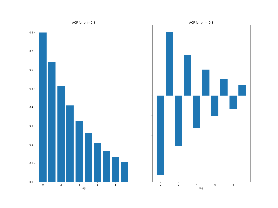
$$\begin{align} \rho_{l} &= \begin{cases} 1,~~~~ l=0 \\ \phi_{1}\rho_{l-1},~~~~ l>0 \end{cases} \end{align}$$

For $\rho > 0$, the ACF of a AR(1) series decays exponentially with rate $\phi_1$. While for a negative $\rho$, the plot consists of 2 alternating exponential decays with rate $\phi_{1}^2$.

References:

1. Tsay, Ruey S. Analysis of financial time series, 3rd edition. John wiley & sons, 2010.