Convolution Network
In this assignment we are asked to construct a convolution neural network (CNN) without having to worry about optimizing it. This is a great way to understand how CNNs.
The course notes for lecture 5 provide a great visual explanation for how convolution layer transforms an input volume.
Mathematically speaking, given an input image of height \(H\) and width \(W\) and 3 colour planes. Any element of the image can be given as
\[x_{i,j,c} \in \mathbb{R}^{H \times W \times 3}\]Forward Pass
Given an input square image (\(H=W\)) \(X\), a filter \(F\) of dimensions \(f \times f\), zero-padding P and stride \(S\), the dimension of the output will be
\[C = \frac{W - f +2P}{S} + 1\]The output will \(C \times C\) matrix (lets call it \(V\)) and its elements will be given by
\[V_{m,n} = \begin{cases} \label{eqn:convolve} \sum_{i=0}^{f-1} \sum_{j=0}^{f-1} w_{i,j}x_{S*m+i-P, S*n + j-P} + b, \text{where } 0 \leq S*m+i-P < W, 0 \leq S*n + j-P < W \\ 0, \text{otherwise} \end{cases}\]where \(b\) is the scalar bias. We will need to calculate a distinct \(V\) for each filter that we apply to our image. This equation is a mouthful and their are a couple of different ways to write it out in Python, I did it as follows:
def conv_forward_naive(x, w, b, conv_param):
N, C, H, W = x.shape
    F, C, HH, WW = w.shape
    S, P = conv_param['stride'], conv_param['pad']
    output_d = (W - HH + 2*P)/S + 1
    print(output_d)
    # To make sure that dimensions work out
    assert output_d == int(output_d)

    output_d = int(output_d)

    output_volume = (N, F, output_d, output_d)

    V = np.zeros(output_volume)

    X = np.zeros((N, C, H+2*P, W+2*P))

    # add padding to x
    for i in range(x.shape[0]):
        for j in range(x.shape[1]):
            X[i][j] = np.pad(x[i][j], P, mode='constant')

    for n in range(N):
        for f in range(F):
            for i in range(output_d):
                for j in range(output_d):
                    # print(X[n, f, S*i: S*i + HH, S*j: S*j + WW] * w[f])
                    V[n, f, i, j] += np.sum(X[n, :, S*i: S*i + HH, S*j: S*j + WW] * w[f]) + b[f]

    out = V

    cache = (x, w, b, conv_param)
    return out, cache
Backward Pass
For the backward pass we need to evaluate
\[\frac{\partial L}{\partial V}\frac{\partial V}{\partial b} \nonumber \\ \frac{\partial L}{\partial V}\frac{\partial V}{\partial w} \nonumber \\ \frac{\partial L}{\partial V}\frac{\partial V}{\partial x} \nonumber \\\]It behooves to actually look at a working matrix to see what the results would look like. I will use the matrix setup given in course notes for lecture 5. A \(5 \times 5\) matrix as input, with padding of 1 and a stride of 2. The output matrix \(V\) would be given as follows
\[\begin{align} \left( \begin{array}{c|c|c} x_{ 0, 0 } w_{ 1,1 }+x_{ 0, 1 } w_{ 1,2 } & x_{ 0, 1 } w_{ 1,0 }+x_{ 0, 2 } w_{ 1,1 } & x_{ 0, 3 } w_{ 1,0 }+x_{ 0, 4 } w_{ 1,1 } \\ +x_{ 1, 0 } w_{ 2,1 }+x_{ 1, 1 } w_{ 2,2 } & +x_{0, 3} w_{1,2}+x_{ 1, 1 } w_{ 2,0 } & +x_{ 1, 3 } w_{ 2,0 }+x_{ 1, 4 } w_{ 2,1 } \\ +b & +x_{ 1, 2 } w_{ 2,1 }+x_{ 1, 3 } w_{ 2,2 } & + b \\ & +b & ~ \\ \hline x_{ 1, 0 } w_{ 0,1 }+x_{ 1, 1 } w_{ 0,2 } & x_{ 1, 1 } w_{ 0,0 }+x_{ 1, 2 } w_{ 0,1 } & x_{ 1, 3 } w_{ 0,0 }+x_{ 1, 4 } w_{ 0,1 } \\ +x_{ 2, 0 } w_{ 1,1 }+x_{ 2, 1 } w_{ 1,2 } & +x_{ 1, 3 } w_{ 0,2 }+x_{ 2, 1 } w_{ 1,0 } & +x_{ 2, 3 } w_{ 1,0 }+x_{ 2, 4 } w_{ 1,1 } \\ +x_{ 3, 0 } w_{ 2,1 }+x_{ 3, 1 } w_{ 2,2 } & +x_{ 2, 2 } w_{ 1,1 }+x_{ 2, 3 } w_{ 1,2 } & +x_{ 3, 3 } w_{ 2,0 }+x_{ 3, 4 } w_{ 2,1 } \\ +b & +x_{ 3, 1 } w_{ 2,0 }+x_{ 3, 2 } w_{ 2,1 } & +b \\ & +x_{ 3, 3 } w_{ 2,2 }+ b & \\ \hline x_{ 3, 0 } w_{ 0,1 }+x_{ 3, 1 } w_{ 0,2 } & x_{ 3, 1 } w_{ 0,0 }+x_{ 3, 2 } w_{ 0,1 } & x_{ 3, 3 } w_{ 0,0 }+x_{ 3, 4 } w_{ 0,1 } \\ +x_{ 4, 0 } w_{ 1,1 }+x_{ 4, 1 } w_{ 1,2 } & +x_{ 3, 3 } w_{ 0,2 }+x_{ 4, 1 } w_{ 1,0 } & +x_{ 4, 3 } w_{ 1,0 }+x_{ 4, 4 } w_{ 1,1 } \\ +b & +x_{ 4, 2 } w_{ 1,1 }+x_{ 4, 3 } w_{ 1,2 } & +b \\ & +b & \end{array}\right) \end{align}\]Their are way too many terms in this matrix but now we can evaluate the derivatives rather easily. Lets proceed
\[\begin{align} \frac{\partial L}{\partial b} &= \frac{\partial L}{\partial V}\frac{\partial V}{\partial b} \nonumber \\ &= \frac{\partial L}{\partial V} \cdot \begin{pmatrix} 1 & 1 & 1 \\ 1 & 1 & 1 \\ 1 & 1 & 1 \end{pmatrix} \nonumber \\ &=\sum_{i=0}^{2} \sum_{j=0}^{2} \left(\frac{\partial L}{\partial V}\right)_{i,j} \end{align}\]Evaluating \(\frac{\partial L}{\partial x}\) is a bit of work but we can deduce some patterns by evaluating a couple elements of the matrix:
\[\begin{align} \frac{\partial L}{\partial x_{0,0}} &= \frac{\partial L}{\partial V}\frac{\partial V}{\partial x_{0,0} } \nonumber \\ &= \frac{\partial L}{\partial V} \cdot \begin{pmatrix} w_{1,1} & 0 & 0 \\ 0 & 0 & 0 \\ 0 & 0 & 0 \end{pmatrix} \nonumber \\ &= \left(\frac{\partial L}{\partial V}\right)_{0,0}w_{1,1} \end{align}\] \[\begin{align} \frac{\partial L}{\partial x_{1,0}} &= \frac{\partial L}{\partial V}\frac{\partial V}{\partial x_{1,0} } \nonumber \\ &= \frac{\partial L}{\partial V} \cdot \begin{pmatrix} 0 & 0 & 0 \\ w_{0,1} & 0 & 0 \\ 0 & 0 & 0 \end{pmatrix} \nonumber \\ &= \left(\frac{\partial L}{\partial V}\right)_{0,0}w_{0,1} \end{align}\] \[\begin{align} \frac{\partial L}{\partial x_{1,1}} &= \frac{\partial L}{\partial V}\frac{\partial V}{\partial x_{1,0} } \nonumber \\ &= \frac{\partial L}{\partial V} \cdot \begin{pmatrix} w_{2,2} & w_{2,0} & 0 \\ w_{0,2} & w_{0,0} & 0 \\ 0 & 0 & 0 \end{pmatrix} \nonumber \\ &= \left(\frac{\partial L}{\partial V}\right)_{0,0}w_{2,2} + \left(\frac{\partial L}{\partial V}\right)_{0,1}w_{2,2} +\left(\frac{\partial L}{\partial V}\right)_{1,0}w_{0,2} + \left(\frac{\partial L}{\partial V}\right)_{1,1}w_{0,0} \end{align}\]With a bit of reasoning combined with a lot of trial and error, we can deduce that a general solution will look as follows
\[\begin{align} \frac{\partial L}{\partial x_{i,j}} &= \frac{\partial L}{\partial V}\frac{\partial V}{\partial x_{i,j} } \nonumber \\ &= \sum_{w1=0}^{2} \sum_{w2=0}^{2}\sum_{k=\text{max}(0, w1*S - P)}^{\text{min}(w1*S + f - P, W)} \sum_{l=\text{max}(0, w2*S - P)}^{\text{min}(w2*S + f - P, W)} \left(\frac{\partial L}{\partial V}\right)_{w1,w2}w_{i+P-w1*S,j+P-w2*S} \end{align}\]To evaluate \(\frac{\partial L}{\partial w}\) I used the same strategy that worked for me previously, I calculated a couple of elements of the matrix and found some patterns to determine the general solution.
\[\begin{align} \frac{\partial L}{\partial w_{0,0}} &= \frac{\partial L}{\partial V}\frac{\partial V}{\partial w_{0,0} } \nonumber \\ &= \frac{\partial L}{\partial V} \cdot \begin{pmatrix} 0 & 0 & 0 \\ 0 & x_{1,1} & x_{1,3} \\ 0 & x_{3,1} & x_{3,3} \end{pmatrix} \nonumber \\ &= \left(\frac{\partial L}{\partial V}\right)_{1,1}x_{1,1} + \left(\frac{\partial L}{\partial V}\right)_{1,2}x_{1,3} + \left(\frac{\partial L}{\partial V}\right)_{2,1}x_{3,1} + \left(\frac{\partial L}{\partial V}\right)_{2,2}x_{3,3} \end{align}\] \[\begin{align} \frac{\partial L}{\partial w_{1,0}} &= \frac{\partial L}{\partial V}\frac{\partial V}{\partial w_{1,0} } \nonumber \\ &= \frac{\partial L}{\partial V} \cdot \begin{pmatrix} 0 & x_{1,0} & 0 \\ x_{2,1} & x_{1,1} & x_{2,3} \\ 0 & x_{4,1} & x_{4,3} \end{pmatrix} \nonumber \\ =& \left(\frac{\partial L}{\partial V}\right)_{0,1}x_{1,0} + \left(\frac{\partial L}{\partial V}\right)_{1,0}x_{2,1} + \left(\frac{\partial L}{\partial V}\right)_{1,1}x_{1,1} + \left(\frac{\partial L}{\partial V}\right)_{1,2}x_{2,3} \\ &+ \left(\frac{\partial L}{\partial V}\right)_{2,1}x_{4,1} + \left(\frac{\partial L}{\partial V}\right)_{2,2}x_{4,3} \end{align}\]The general solution is
\[\begin{align} \frac{\partial L}{\partial w_{i,j}} = \begin{cases} \sum_{w1=0}^{2} \sum_{w2=0}^{2} w_{w1, w2} x_{S*w1 + i, S*w2 + j}, \text{ where }0 \leq S*w1 + i < W, 0 \leq S*w2 + j < W \\ 0, \text{ otherwise} \end{cases} \end{align}\]Their must be a way to simpify these equations and write them in a more efficient manner but that is outside the scope of this assignment. Here is the naive Python implementation of the results derived in this section:
def conv_backward_naive(dout, cache):
    x, w, b, conv_param = cache
    N, C, H, W = x.shape
    F, C, HH, WW  = w.shape
    S, P = conv_param['stride'], conv_param['pad']
    output_d = (W - HH + 2 * P) / S + 1
    # To make sure that dimensions work out
    if output_d == int(output_d):
        output_d = int(output_d)
    else:
        return

    X = np.zeros((N, C, H + 2, W + 2))

    # add padding to x
    for i in range(x.shape[0]):
        for j in range(x.shape[1]):
            X[i][j] = np.pad(x[i][j], 1, mode='constant')

    # Number of b is equivalent to the number of filters
    db = np.zeros(F)
    for f in range(F):
        for n in range(N):
            db[f] += np.sum(dout[n, f, : ,:])

    dw = np.zeros((F, C, HH, WW))
    for c in range(C):
        for f in range(F):
            for i in range(WW):
                matrix_elements_i = np.array( [[S*i_ + i] * output_d for i_ in range(output_d)] )
                for j in range(HH):
                    matrix_elements_j = np.array( [[S*i_ + j]*output_d for i_ in range(output_d)] ).T
                    dw[f, c, i, j] += np.sum(dout[:, f, :, :] * X[:, c, matrix_elements_i, matrix_elements_j])

    dx = np.zeros((N, C, H, W))
    for f in range(F):
        for c in range(C):
            for n in range(N):
                for w1 in range(output_d):
                    for w2 in range(output_d):
                        for i in range( max(0, w1*S - P), min(W, w1*S + WW - P) ):
                            for j in range( max(0, w2*S - P), min(H, w2*S + HH - P) ):
                                dx[n, c, i, j]+=np.sum(dout[n, f, w1, w2] * w[f, c, i + P - w1*S, j + P - w2*S])

    return dx, dw, db
Max Pooling
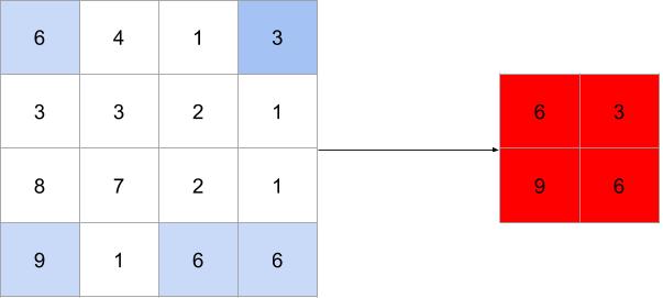
Pooling is conceptually very simple. In forward pooling we run our filter over the image and select the max value in the window only. Forward max pooling with a \(2 \times 2\) filter and a stride of 2 would look as follows:
 Forward max pooling with a \(2 \times 2\) filter and a stride of 2
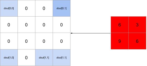
While the backward pass over this pooling will be
 Backward pass over max pooling with a \(2 \times 2\) filter and a stride of 2
If you are interested in more details check out this blog post by Lanston Chu.
Now for the code
def max_pool_forward_naive(x, pool_param):
    out = None

    N, C, H, W = x.shape
    pool_height, pool_width, S = pool_param['pool_height'], pool_param['pool_width'], pool_param['stride']

    H_pool = (H - pool_height)//S + 1
    W_pool = (W - pool_width)//S + 1
    out = np.zeros((N, C, H_pool, W_pool))

    for n in range(N):
        for c in range(C):
            for i in range(H_pool):
                pool_i = np.array([[i_]*pool_height for i_ in range(i*S, i*S + pool_height)])
                for j in range(W_pool):
                    pool_j = np.array([[j_]*pool_width for j_ in range(j*S, j*S + pool_width)]).T
                    out[n,c,i,j] = np.max(x[n,c, pool_i, pool_j])

    cache = (x, pool_param)
    return out, cache

def max_pool_backward_naive(dout, cache):
    dx = None
    x, pool_param = cache

    N, C, H, W = x.shape
    pool_height, pool_width, S = pool_param['pool_height'], pool_param['pool_width'], pool_param['stride']

    H_pool = (H - pool_height) // S + 1
    W_pool = (W - pool_width) // S + 1

    dx = np.zeros((N, C, H, W))

    for n in range(N):
        for c in range(C):
            for i in range(H_pool):
                pool_i = np.array([[i_] * pool_height for i_ in range(i * S, i * S + pool_height)])
                for j in range(W_pool):
                    pool_j = np.array([[j_] * pool_width for j_ in range(j * S, j * S + pool_width)]).T
                    max_val = np.amax(x[n,c, pool_i, pool_j])
                    for h in range(i * S, i * S + pool_height):
                        for w in range(j * S, j * S + pool_width):
                            dx[n, c, h, w] += dout[n, c, i, j] * int(x[n, c, h, w] >= max_val)

    return dx
Spatial and Group Batch Normalization
Spatial and Group Batch Normalization are very similar to Group Normalization and Layer Normalization covered in the previous assignment. Only now we are dealing with 3-dimensional matrices instead of 2.
Check out the full assignment here
Comments